6 The pipeline
- RStudio Environment. Let’s rearrange the panel layout:
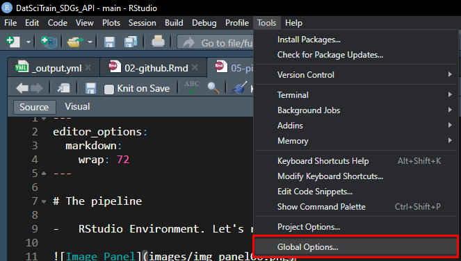
Tools>Global Options…
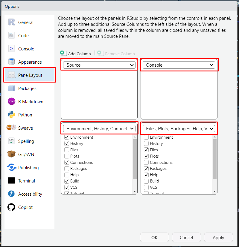
Pane Layout
6.1 Essential data management and folder structure
├── config.R
├── data_derived
│   ├── Australia_SDG_14.csv
│   ├── sdg_14.csv
│   ├── sdg_14_unclos_map.csv
│   └── sdg_3_1_2.csv
├── data_provided
│   ├── country-to-region-mapping.csv
│   ├── Ocean Accounts Diagnostic Tool_formatted.pdf
│   ├── SDG-DSD-Guidelines.pdf
│   ├── SDG.xlsx
│   └── SDG_Updateinfo.xlsx
├── DatSciTrain_SDGs_API_R.Rproj
├── figures_and_tables
│   ├── fig2.png
│   └── sdg14_Australia.docx
├── LICENSE
├── R
│   ├── do_clean.R
│   ├── do_get_sdg_api.R
│   ├── do_map.R
│   ├── do_plot.R
│   └── do_tab_Australia.R
├── README.md
└── run.R
6.2 config.R
# packages

if (!require(data.table)) {
  install.packages("data.table")
  library(data.table)
}

if (!require(ggplot2)) {
  install.packages("ggplot2")
  library(ggplot2)
}

if (!require(sf)) {
  install.packages("sf")
  library(sf)
}

if (!require(RColorBrewer)) {
  install.packages("RColorBrewer")
  library(RColorBrewer)
}

if (!require(rnaturalearth)) {
  install.packages("rnaturalearth")
  library(rnaturalearth)
}

if (!require(rnaturalearthdata)) {
  install.packages("rnaturalearthdata")
  library(rnaturalearthdata)
}

## set folder names
folder_names <- c("data_derived", "data_provided", "figures_and_tables")

for (folder_name in folder_names) {
  if (!dir.exists(folder_name)) {
    dir.create(folder_name)
    cat("Folder", folder_name, "created.\n")
  } else {
    cat("Folder", folder_name, "already exists.\n")
  }
}

## source functions
file_list <- list.files(path = "R", pattern = "\\.R$", full.names = TRUE)

# Source each .R file
for (file in file_list) {
  source(file)
}
6.3 run.R
source("config.R")

### 1. Download ####
# Use the function to download SDGs data
do_get_sdg_api()

### 2. Data cleaning ####
# Function to clean the data downloaded
indat <- do_clean()

### 3. Tabulating ####
tab <- do_tab_country(indat, country = "Indonesia")

### 4. Visualise ####
# Generate and interactive plot with the data cleaned
do_plot()

### 5. Map ####
do_map()
6.4 do_get_sdg_api
do_get_sdg_api <- function(
    output = "data_derived/sdg_14.csv"
){
  # (Client URL) command line tool that enables data exchange between a device
  # and a server through a terminal
  curl <- paste0(
    'curl -X POST --header "Content-Type: application/x-www-form-urlencoded" ',
    '--header "Accept: application/octet-stream" ',
    '-d "goal=14" ',
    '"https://unstats.un.org/sdgapi/v1/sdg/Goal/DataCSV" -o',
    output)

  # Execute cURL
  system(curl)
}
6.5 do_clean
do_clean <- function() {
  # options(scipen = 1000)
  # Load data
  indat <- fread(file.path("data_derived", "sdg_14.csv"))
  # mapping  <- fread(file.path("data_provided", "country-to-region-mapping.csv"))

  # Keep only the values that are either blank or 'A' under 'Observation Status', drop the rest
  indat <- indat[`[Observation Status]` == "" | `[Observation Status]` == "A"]

  # Replace '-' with '_' across all disaggregation values
  cols_to_replace <- grep("\\[.*\\]",
                          names(indat),
                          value = TRUE)
  indat[, (cols_to_replace) := lapply(.SD, function(x) gsub("-", "_", x)),
        .SDcols = cols_to_replace]
  return(indat)
}
6.6 do_tab_country
do_tab_country <- function(
    indat,
    country
){
# Filter the input data for the specified country
foo <- indat[GeoAreaName == country]

# Select specific columns from the filtered data
foo14 <- foo[, .(Indicator,
                 SeriesDescription,
                 TimePeriod,
                 Source)]

# Convert TimePeriod column to numeric for easier calculations
foo14[, NumericTimePeriod := as.numeric(TimePeriod)]

# Calculate min and max year for each SeriesDescription using TimePeriod
time_ranges <- foo14[, .(
  StartYear = min(NumericTimePeriod, na.rm = TRUE),
  EndYear = max(NumericTimePeriod, na.rm = TRUE)
), by = SeriesDescription]

# Create a time range string (e.g., "2000-2020" or "2000" if start and end year are the same)
time_ranges[, TimeRange := ifelse(StartYear == EndYear, as.character(StartYear), paste(StartYear, EndYear, sep = "-"))]

# Merge the new time range back to the main data.table
foo14 <- merge(foo14, time_ranges, by = "SeriesDescription", all.x = TRUE)

# Drop temporary columns that are no longer needed
foo14[, NumericTimePeriod := NULL]
foo14[, StartYear := NULL]
foo14[, EndYear := NULL]
foo14[, TimePeriod := NULL]

# Keep unique rows based on SeriesDescription
unq <- unique(foo14, by = "SeriesDescription")

# Select the final columns to include in the output
unq <- unq[, .(Indicator, SeriesDescription, TimeRange, Source)]

# Define the output file name based on the country
out_name <- paste0("data_derived/", country, "_SDG_14.csv")

# Write the data to a CSV file
fwrite(unq, out_name)

return(unq)
}
6.7 do_plot
do_plot <- function(){

  # Subset the data to only include rows where the Indicator is "14.7.1"
  sdg1471 <- indat[Indicator=="14.7.1"]

  # Order the subsetted data by GeoAreaName in ascending order
  sdg1471 <- sdg1471[order(sdg1471$GeoAreaName, decreasing = FALSE)]

  # Display the unique GeoAreaNames in the subsetted and ordered data
  unique(sdg1471$GeoAreaName)

  # Further subset the data to only include rows where the GeoAreaName is "Indonesia"
  sdg1471_ind <- sdg1471[GeoAreaName=="Indonesia"]

  # Let's make a simple plot using base R
  plot(
    sdg1471_ind$TimePeriod,
    sdg1471_ind$Value
  )

  # Some improvements:
  # type = "l"
  # col = "blue"
  # lwd = 2
  # main = "Sustainable Fisheries as a proportion of GDP in Indonesia"
  # xlab = "Year"
  # ylab = "(%)"

  # Comparing Indonesia with other countries, subsetting first
  sdg1471_comp <- sdg1471[GeoAreaName %in% c("Indonesia", "Malaysia", "Cook Islands")]

  # Create the plot using ggplot2
  ggplot(sdg1471_comp,
         aes(x = TimePeriod, y = Value, color = GeoAreaName, group = GeoAreaName)) +
    geom_line(size = 1.2) +
    labs(title = "Sustainable Fisheries as a proportion of GDP",
         x = "Year",
         y = "(%)",
         color = "Country") +
    theme_minimal()

  # Include world averages for comparison
  sdg1471_comp_two <- sdg1471[GeoAreaName %in% c("Indonesia", "Malaysia", "Cook Islands", "World")]

  # Create the plot using ggplot2
 p <-  ggplot(sdg1471_comp_two,
         aes(x = TimePeriod, y = Value, color = GeoAreaName, group = GeoAreaName)) +
    geom_line(size = 1.2) +
    labs(title = "Sustainable Fisheries as a proportion of GDP (including World average)",
         x = "Year",
         y = "(%)",
         color = "Country") +
    theme_minimal()

return(p)
}
6.8 do_map
do_map <- function()
{
# United Nations Convention on the Law of the Sea (UNCLOS)

  # Indicator 14.c.1: Number of countries making progress in ratifying,
  # accepting and implementing through legal, policy and institutional frameworks,
  # ocean-related instruments that implement international law, as reflected in
  # the United Nations Convention on the Law of the Sea, for the conservation and
  # sustainable use of the oceans and their resources

foo <- indat[SeriesCode == "ER_UNCLOS_RATACC" | SeriesCode == "ER_UNCLOS_IMPLE"]

foo1 <- foo[SeriesCode == "ER_UNCLOS_RATACC", .SD[which.max(as.numeric(TimePeriod))], by = GeoAreaName]

foo2<- foo[SeriesCode == "ER_UNCLOS_IMPLE", .SD[which.max(as.numeric(TimePeriod))], by = GeoAreaName]

# Get country polygons
world <- rnaturalearth::ne_countries(scale = "medium", returnclass = "sf")

setnames(foo1, "GeoAreaName", "name")
setnames(foo2, "GeoAreaName", "name")

foo2_names <- unique(foo2$name)
foo1_names <- unique(foo1$name)
world_names <- unique(world$name)
names_diff_foo2_world <- setdiff(foo2_names, world_names)
names_diff_foo1_world <- setdiff(foo1_names, world_names)

print("Names in foo2 not in world:")
print(names_diff_foo2_world)
print(names_diff_foo1_world)

foo2[name == "Republic of Korea", name := "South Korea"]
foo2[name == "United Kingdom of Great Britain and Northern Ireland", name := "United Kingdom"]
foo2[name == "Russian Federation", name := "Russia"]
foo2[name == "Venezuela (Bolivarian Republic of)", name := "Venezuela"]

foo1[name == "Republic of Korea", name := "South Korea"]
foo1[name == "United Kingdom of Great Britain and Northern Ireland", name := "United Kingdom"]
foo1[name == "Russian Federation", name := "Russia"]
foo1[name == "Venezuela (Bolivarian Republic of)", name := "Venezuela"]

foo2_imple <- foo2[SeriesCode == "ER_UNCLOS_IMPLE"]
foo1_rat <- foo1[SeriesCode == "ER_UNCLOS_RATACC"]

foo3 <- rbind(foo2_imple, foo1_rat)

foo3_map <- merge(world, foo3, by = "name", all.x = TRUE, fill = TRUE)

setDT(foo3_map)

# Replace NaN and NA in 'Value' with NA for uniform handling
foo3_map[, Value := fifelse(is.nan(Value) | is.na(Value), as.numeric(NA), Value)]

foo3_map[, ValueFactor := cut(Value, breaks = c(0, 50, 69, 79, 89, 100),
                              include.lowest = TRUE, right = TRUE,
                              labels = c("0-50%", "51-69%", "70-79%", "80-89%", "90-100%"))]

foo4 <- foo3_map[!is.na(foo3_map$Value)]
foo5 <- foo4[, c("name", "Value", "Indicator", "TimePeriod", "SeriesDescription"), drop = FALSE]
write.csv(foo5, "data_derived/sdg_14_unclos_map.csv", row.names = FALSE)

foo3_map <- st_as_sf(foo3_map)

equal_earth_projection <- st_crs("+proj=eqearth +datum=WGS84")

p <- ggplot(data = foo3_map) +
  geom_sf(aes(geometry = geometry, fill = ValueFactor), color = "white", size = 0.2) +
  scale_fill_brewer(palette = "YlGnBu", name = "", na.value = "grey") +
  coord_sf(crs = equal_earth_projection, datum = NA) +  # Apply Equal Earth projection
  theme(
    panel.background = element_rect(fill = "white"),
    legend.position = "top"
  )

ggsave("figures_and_tables/fig_map.png", plot = p, width = 10, height = 6, dpi = 300, units = "in")

}